If you are streaming financial market data you will quickly accumulate a large amount of tick data which will start to consume large amounts of storage. Often it’s desirable to resample the data to a format that will be easier to store

One possible solution is to deploy micro services to stream data into InfluxDB. We are not going to be talking about those components in this article. In this article we discuss how we can use the stream data processing task features from InfluxDB and the Flux language to process market data into more manageable OHLC (Open, High, Low, Close) data bars. We will also discuss some of the initial setup steps required to get InfluxDB up and running as it will help later to have that knowledge when we dive into the data sampling and the terminology used there.

If you have ever used InfluxDB before you have probably used the TICK stack from InfluxDB v1. With the introduction of the InfluxDB v2 platform InfluxData introduced a platform in a single binary which makes setup and configuration much easier especially using Docker containers. This article is going to assume you already have Docker and Docker Compose tools installed. If you need to do that head over to https://docs.docker.com/get-docker and install those first

InfluxData hosts Docker containers for InfluxDB at https://quay.io/influxdb/influxdb

At the time of writing this article the latest version available was v2.0.4. Once you have Docker setup it’s simple to spin up an instance of InfluxDB v2 using a Docker compose file to grab the container from quay.io and run it

There’s not much to getting things setup as you can see. A couple of interesting parts are the volume mapping from the container to the host that allows data to persist between runs of the database so we don’t have it reset every time. We also expose port 8086 so we can communicate with the InfluxDB API. If you run this config with Docker compose you will be able to visit http://localhost:8086 and you should see the initial InfluxDB welcome page

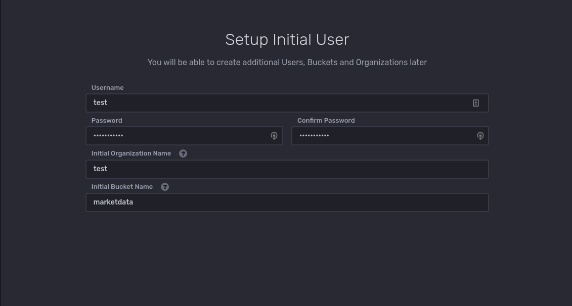
The next step is to setup the initial database parameters by providing and organization name and a data bucket name. The data bucket is where you store your time series data. For this article we are going to be using the organization ‘test’ and our initial data bucket will be called ‘marketdata’

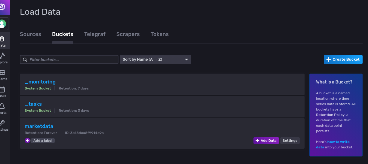
After setting that up you can view the ‘Data’ panel and you should see the bucket listed. The default retention policy is forever which is fine for our test. The retention policy can easily be modified, to 30 days for example.

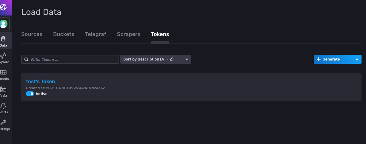
InfluxDB API calls require a token and you can find this token in the same ‘Data’ section under ‘Tokens’. This token will need to be passed to your code making the API calls to InfluxDB.

One way to do this for development purposes is to create an environment variable section in your Docker compose file for the service that’s going to call the API

You can then use this API token with one of the InfluxDB client libraries to send data to be ingested. There are client libraries for many languages here https://docs.influxdata.com/influxdb/cloud/tools/client-libraries

E.g. For exmple in Golang you could write data using your token into the ‘marketdata’ bucket for organization ‘test’ like this

client := influxdb2.NewClient("http://localhost", DB_TOKEN)

writeAPI := client.WriteAPIBlocking("test", "marketdata")

It’s as easy as that! Once you have written some data out you will be able to view the measurements via the Influx UI

Okay so at this point we are going to assume that the InfluxDB is up and running and there is some service that is sending some tick data to be ingested by the database using the InfluxDB API. Now we can look at how to use Flux to resample that data. Flux is designed for querying, analyzing, and acting on data. This data comes from buckets. We setup a test bucket previously during database setup so that’s what we will use here.

You tell Flux which bucket to use by using the from() function

dataset = from(bucket: “test")

You also need to specify a time range for the data query. A time range is required so that the query to InfluxDB isn’t unbounded as that can be unlimited in size. We will specify a start of the range to be 3 minutes ago

dataset = from(bucket: “marketdata")

|> range(start: -3)

Each bucket has measurements that acts as a container for tags, fields, and timestamps. A measurement name should describe your data. We chose to have a measurement name of ‘tradedata’ which is set when the market data service sends data to be ingested over the API. We need to tell the Flux query that we are interested in this measurement. The Flux filter function filters data based on conditions defined in a predicate function (fn)

filter(fn: (r) =>

(r["_measurement"] == “tradedata"))

For our OHLC calculation we are going to grab the ‘Last’ field that we stored in our time series data and also the ‘Size’ field to keep a track of the volume.

filter(fn: (r) =>

(r["_field"] == "Size" or r["_field"] == “Last"))`}

So putting it all together we have our first part of our Flux program complete to extract a new table of results with just the data that we need for the OHLC calculations

dataset = from(bucket: “test")

|> range(start: -3)

|> filter(fn: (r) =>

(r["_measurement"] == “tradedata"))

|> filter(fn: (r) =>

(r["_field"] == "Size" or r["_field"] == “Last"))

The next step will be to start calculating the OHLC values from the ‘Last’ field values. We are going to create one minute OHLC bars. This is where the InfluxDB Flux functions are so powerful. We can pass the table ‘dataset’ as an input to an aggregation function that will use the Flux functions first(), max(), min() and last() to calculate the open, high, low and close values. The aggregation function works on a fixed window of time. In our case we will use a one minute window.

For example, to get the first value from our ‘Last’ values during a one minute window we would use the Flux aggregateWindow

dataset |> filter(fn: (r) =>

(r["_field"] == "Last"))

|> aggregateWindow(every: 1m, fn: first)`

Because we want to create a new data set and place it into a different bucket from the original tradedata bucket an additional step is required to map records from the input table to new table and then output those value to the new bucket. Because in this step we’re getting the first value this will be the ‘open’ value for our OHLC records. So we map the value to the ‘open’ field in the new table

|> map(fn: (r) =>\n\t({ _time: r._time, _field: "open", _measurement: r._measurement, _value: r._value, topic: r.topic, symbol: r.symbol, })) |> limit(n: 3) |> to(bucket: "ohlc_1m_data", org: "test")

Remember this is only the ‘open’ part of the OHLC data. The calculations logic for the rest of the OHLC data is essentially the same apart from we swap out the function passed to the aggregateWindow function and write a different field in the mapping. Adding all of the code here would make this article way too long, so you can find the complete Flux script over at our Github page InfluxDB OHLC Flux Code

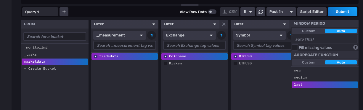
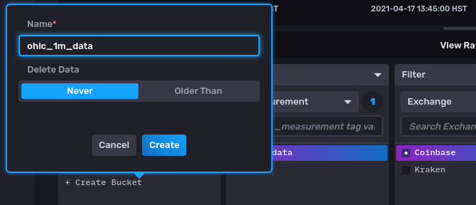
Now we are going to add the Flux script to our InfluxDB. The first step is to create a new bucket to hold the one minute data that our script is going to generate. We can do this via the InfluxDB API or via the InfluxDB UI. We will use the UI here. Go to the ‘Explore’ tab and find the option ‘Create Bucket’

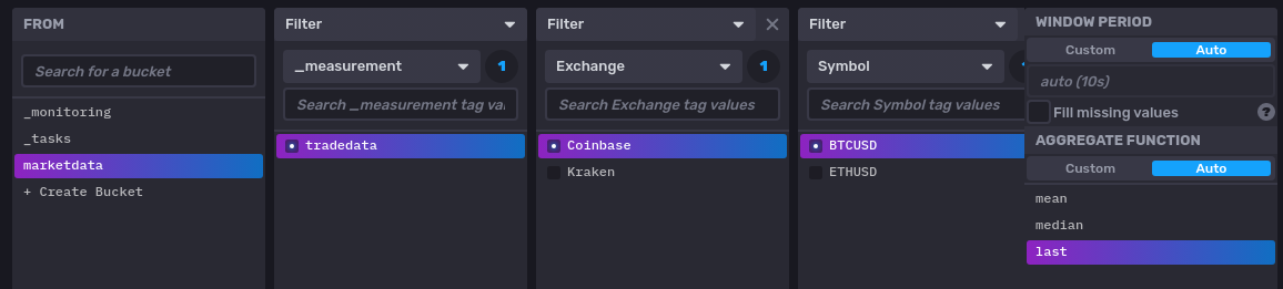
We are going to call our bucket ‘ohlc_1m_data’

Next go to the ‘Tasks’ tab, create a new task, paste in the Flux code and save it. For the scheduling we setup the Cron parameter to be */1 * * * 1-5 which in English means ‘At every minute on every day-of-week from Monday through Friday’

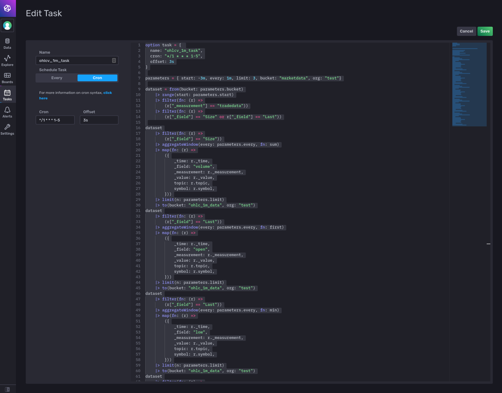Once you have created the task, InfluxDB will add a block into your script with the Cron task parameters included

When you run the task InfluxDB will execute it according to the Cron job and OHLC data will start to be generated, in this case every minute. You can see the data by going to the ‘Explore’ tab and selecting the ‘ohlc_1m_data’ bucket.

Hopefully this article has been a good introduction to using the powerful InfluxDB Flux features. We are really only just scratching the surface with the Flux capabilities in this article. Head over to the official InfluxDB Flux docs here to take a deeper dive